PCA, SVD and Eigen decomposition
Principal component analysis (PCA) is a popular method for dimensional reduction, and has been invented independently many times in different fields, resulting in various definitions. This note attempts to unify 2 of the most popular definitions of principal components and illustrate how PCA can be done correspondingly.
Alternative definitions
PCA from the SVD of the centered matrix
The singular value decomposition (SVD) of an \(n\times d\) matrix \(X\) has the form
\[ X = U_X\Sigma_X V^T_X \]
Let \(Y\) the centered version of \(X\), such that all the columns of \(Y\) have zero mean. The SVD of \(Y\) gives the principal components of \(X\)
\[ Y = U_Y \Sigma_Y V^T_Y \] The rows of \(V^T\) (i.e. columns of \(V\)) are called the principal components of \(X\).
PCA from the eigen decomposition of the covariance matrix
Alternatively, the eigen decomposition of \(X^TX\) (also of the covariance matrix \(S = X^T X / n\), up to a factor \(n\))
\[ X^TX = VD^2 V^T \]
The derived variable \(z_i = X v_i = u_i d_i\) is called the i-th principal component of \(X\), with the variance
\[ Var(z_i) = Var(X v_i) = \frac{d^2_i}{n} \]
Computing the principal components
From the definitions above, it follows that we can compute principal components using either SVD or eigen decomposition. SVD is usually the preferred method due to better numerical accuracy. The codes below illustrate 3 different methods to compute the principal components:
- SVD on the column-centered matrix \(Y\)
- Eigen decomposition of \(X^TX\)
- Using the built-in R function
prcomp()which uses the SVD, but the variance estimate uses \(n-1\) instead of \(n\)
Simulation data
n = 20
x = mvrnorm(n, c(2,-1,0), matrix(c(1, 0.95, 0.7, 0.95, 1, 0.5, 0.7, 0.5, 1), 3, 3))
y = scale(x, center=TRUE, scale=FALSE)
mean_y = apply(y,1,mean)

# Computing PC by SVD
s = svd(y)
pc.s = sweep(s$u,MARGIN = 2,STATS = s$d, FUN = '*') # XV = UD, UD is more efficient to compute
# pc.s = y %*% s$v

# Computing PCs by eigen decomposition
covmat = t(y) %*% y / nrow(y)
eig = eigen(covmat)
pc.e = y %*% eig$vectors

# Computing PC using built-in R function
prc = prcomp(y,center=FALSE,scale=FALSE)
rotation = prc$rotation
pc.r = y %*% rotation
Rotated data points
data.frame('PC1' = pc.s[,1], 'PC2' = pc.s[,2], 'mean' = mean_y, 'method'='svd') %>%
    rbind(data.frame('PC1' = pc.e[,1], 'PC2' = pc.e[,2], 'mean' = mean_y, 'method' = 'eigen')) %>%
    rbind(data.frame('PC1' = pc.r[,1], 'PC2' = pc.r[,2], 'mean' = mean_y, 'method' = 'prcomp')) %>%
    ggplot() +
    facet_grid( . ~ method) +
    geom_point(aes(x=PC1,y=PC2,color=mean))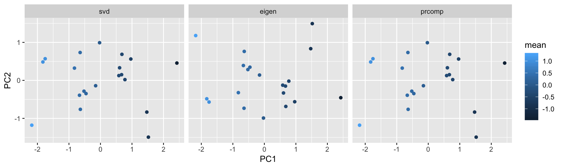
Percentage of variance explained by each principal component
varExplained.s = (s$d^2)/sum(s$d^2)
varExplained.e = (eig$values / sum(eig$values))
varExplained.r = (prc$sdev^2)/sum(prc$sdev^2)
data.frame('svd' = varExplained.s,
           'eigen' = varExplained.e,
           'prcomp' = varExplained.r) %>%
    cbind('index' = 1:length(varExplained.e)) %>%
    reshape2::melt(id.vars = 'index') %>%
    ggplot() +
    geom_point(aes(x=index,y=value,group=variable,color=variable,shape=variable)) +
    geom_line(aes(x=index,y=value,group=variable,color=variable),alpha=0.5) +
    ylab('Percentage of variance explained')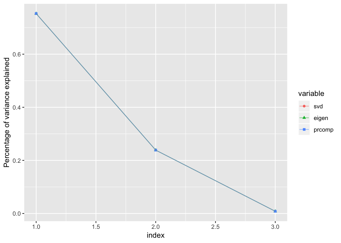
Variance of the principal component \(z_i\)
var.s = (s$d)^2/nrow(y)
var.s1 = (s$d)^2/(max(1,nrow(y) -1)) # this is the formula used by prcomp
var.e = (eig$values)
var.r = (prc$sdev^2)
data.frame('svd' = var.s,
           'svd.1' = var.s1,
           'eigen' = var.e,
           'prcomp' = var.r) %>%
    cbind('index' = 1:length(var.s)) %>%
    reshape2::melt(id.vars = 'index') %>%
    ggplot() +
    geom_point(aes(x=index,y=value,group=variable,color=variable,shape=variable)) +
    geom_line(aes(x=index,y=value,group=variable,color=variable)) +
    ylab('Variance')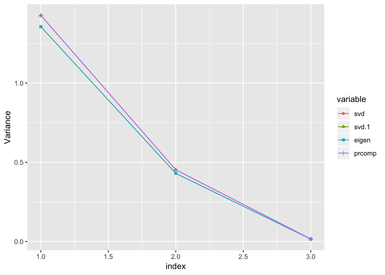
Iris data set
data(iris)
y = scale(iris[,c(1:4)], center =TRUE, scale = TRUE)
mean_y = apply(y,1,mean)

# Computing PC by SVD
s = scale(y, center=TRUE, scale = FALSE) %>%
    svd()
pc.s = sweep(s$u,MARGIN = 2,STATS = s$d, FUN = '*')

# Computing PCs by eigen decomposition
covmat = t(y) %*% y / nrow(y)
eig = eigen(covmat)
pc.e = y %*% eig$vectors

# Computing PC using built-in R function
prc = prcomp(y,center=FALSE,scale=FALSE)
rotation = prc$rotation
pc.r = y %*% rotation
Rotated data points
data.frame('PC1' = pc.s[,1], 'PC2' = pc.s[,2], 'mean' = mean_y, 'method'='svd') %>%
    rbind(data.frame('PC1' = pc.e[,1], 'PC2' = pc.e[,2], 'mean' = mean_y, 'method' = 'eigen')) %>%
    rbind(data.frame('PC1' = pc.r[,1], 'PC2' = pc.r[,2], 'mean' = mean_y, 'method' = 'prcomp')) %>%
    ggplot() +
    facet_grid( . ~ method) +
    geom_point(aes(x=PC1,y=PC2,color=mean))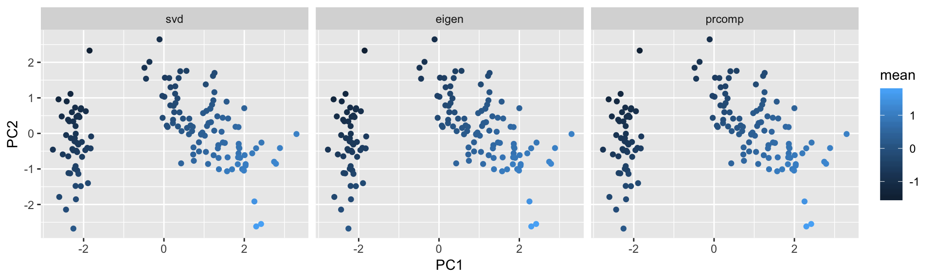
data.frame('PC3' = pc.s[,3], 'PC4' = pc.s[,4], 'mean' = mean_y, 'method'='svd') %>%
    rbind(data.frame('PC3' = pc.e[,3], 'PC4' = pc.e[,4], 'mean' = mean_y, 'method' = 'eigen')) %>%
    rbind(data.frame('PC3' = pc.r[,3], 'PC4' = pc.r[,4], 'mean' = mean_y, 'method' = 'prcomp')) %>%
    ggplot() +
    facet_grid( . ~ method) +
    geom_point(aes(x=PC3,y=PC4,color=mean))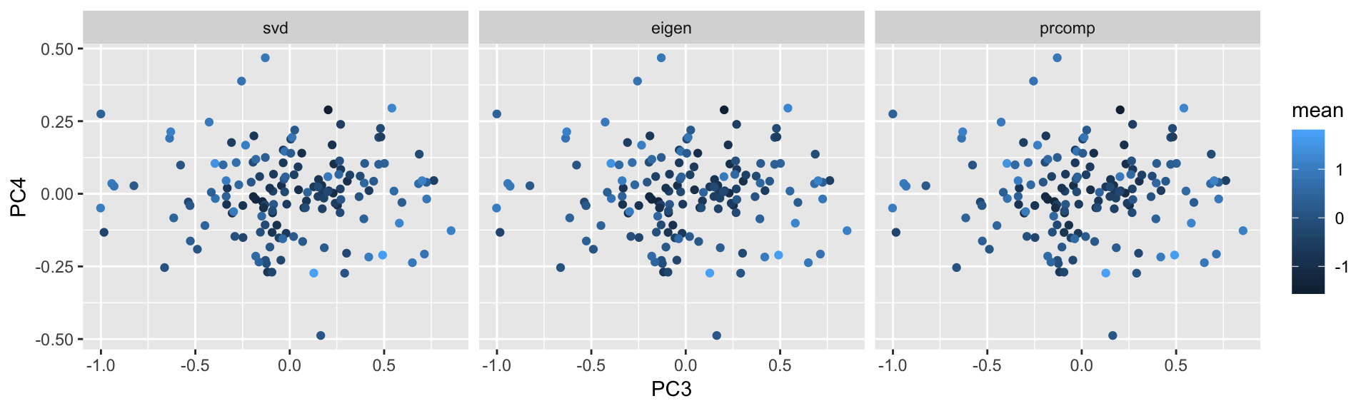
Percentage of variance explained by each principal component
varExplained.s = (s$d^2)/sum(s$d^2)
varExplained.e = (eig$values / sum(eig$values))
varExplained.r = (prc$sdev^2)/sum(prc$sdev^2)
data.frame('svd' = varExplained.s,
           'eigen' = varExplained.e,
           'prcomp' = varExplained.r) %>%
    cbind('index' = 1:length(varExplained.e)) %>%
    reshape2::melt(id.vars = 'index') %>%
    ggplot() +
    geom_point(aes(x=index,y=value,group=variable,color=variable,shape=variable)) +
    geom_line(aes(x=index,y=value,group=variable,color=variable),alpha=0.5) +
    ylab('Percentage of variance explained')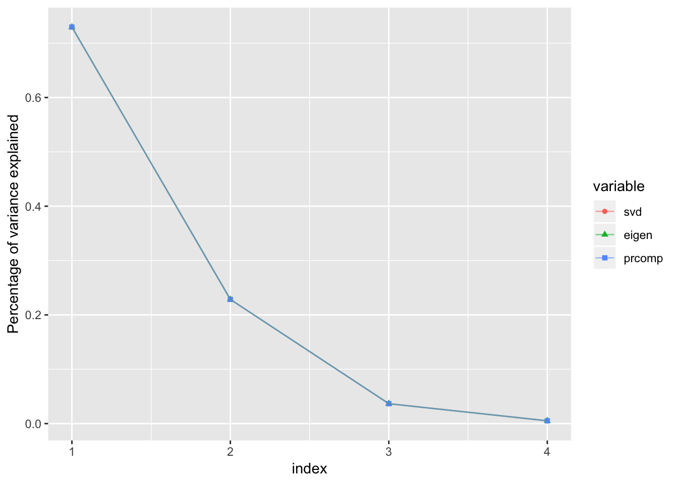
Variance of the principal component \(z_i\)
var.s = (s$d)^2/nrow(y)
var.s1 = (s$d)^2/(nrow(y) -1) # this is the formular used by prcomp
var.e = (eig$values)
var.r = (prc$sdev^2)
data.frame('svd' = var.s,
           'svd.1' = var.s1,
           'eigen' = var.e,
           'prcomp' = var.r) %>%
    cbind('index' = 1:length(var.s)) %>%
    reshape2::melt(id.vars = 'index') %>%
    ggplot() +
    geom_point(aes(x=index,y=value,group=variable,color=variable,shape=variable)) +
    geom_line(aes(x=index,y=value,group=variable,color=variable)) +
    ylab('Variance')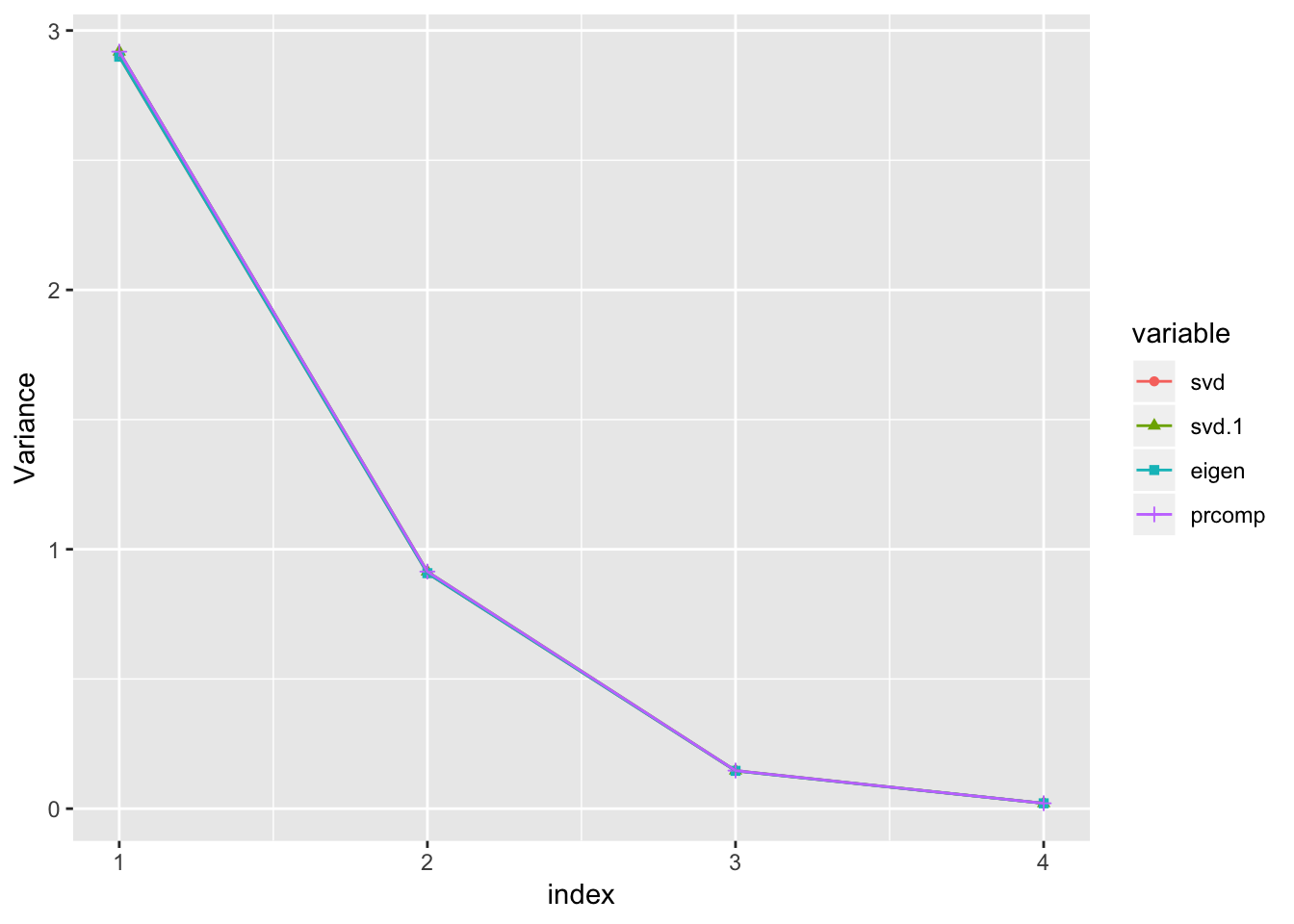
Effects of scaling
n = 20
x = mvrnorm(n, c(2,-1,1), matrix(c(2, 0.95, 0.7, 0.95, 2, 0.5, 0.7, 0.5, 3), 3, 3))
x_center = scale(x, center=TRUE,scale=FALSE)
y = scale(x, center=TRUE, scale=TRUE)
mean_y = apply(y,1,mean)

# Computing PC by SVD
s = svd(x_center)
pc.s = sweep(s$u,MARGIN = 2,STATS = s$d, FUN = '*') # XV = UD, UD is more efficient to compute
# pc.s = y %*% s$v

# Computing PCs by eigen decomposition
covmat = t(x_center) %*% x_center / nrow(x_center)
eig.cov = eigen(covmat)
pc.e1 = x_center %*% eig.cov$vectors

eig.cor = eigen(cor(x))
pc.e2 = x %*% eig.cor$vectors

# Computing PC using built-in R function
prc = prcomp(x,center=TRUE,scale=TRUE)
rotation = prc$rotation
pc.r = x %*% rotation
Rotated data points
data.frame('PC1' = pc.s[,1], 'PC2' = pc.s[,2], 'mean' = mean_y, 'method'='svd') %>%
    rbind(data.frame('PC1' = pc.e1[,1], 'PC2' = pc.e1[,2], 'mean' = mean_y, 'method' = 'eigen-cov-center')) %>%
    rbind(data.frame('PC1' = pc.e2[,1], 'PC2' = pc.e2[,2], 'mean' = mean_y, 'method' = 'eigen-cor-center-scale')) %>%
    rbind(data.frame('PC1' = pc.r[,1],  'PC2' = pc.r[,2], 'mean' = mean_y, 'method' = 'prcomp-center-scale')) %>%
    ggplot() +
    facet_grid( . ~ method) +
    geom_point(aes(x=PC1,y=PC2,color=mean))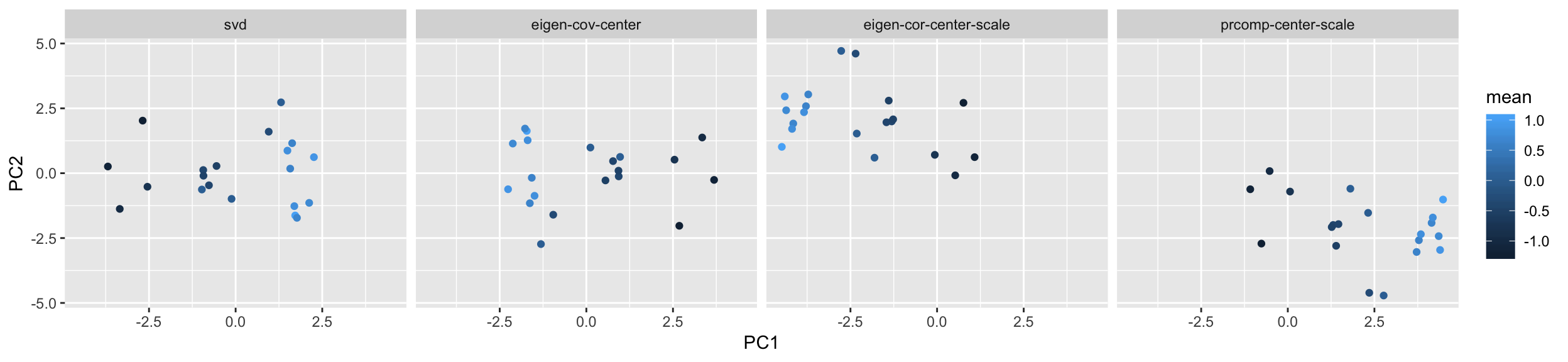
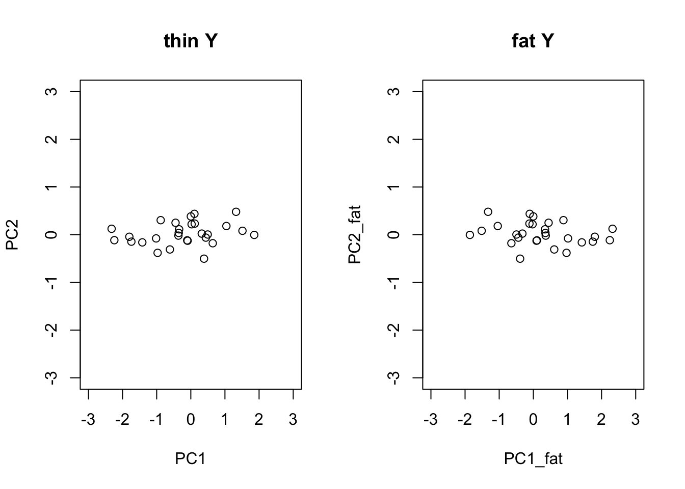
SVD of the thin vs fat matrices
With the data matrix \(Y\) following the convention of rows being observations and columns being dimensions, the i-th principal component of \(Y\) can be obtained from the SVD
\[ Y = UDV^T \]
by
\[ PC_i = U_i \times d_i \] \(U_i\) being the i-th column of \(U\), and \(d_i\) being the i-th singular value.
The thin matrix
n = 30
y = mvrnorm(n, c(0,0), matrix(c(1, 0.95, 0.95, 1), 2, 2))
s = svd(y)
plot.matrix(y,asp=20)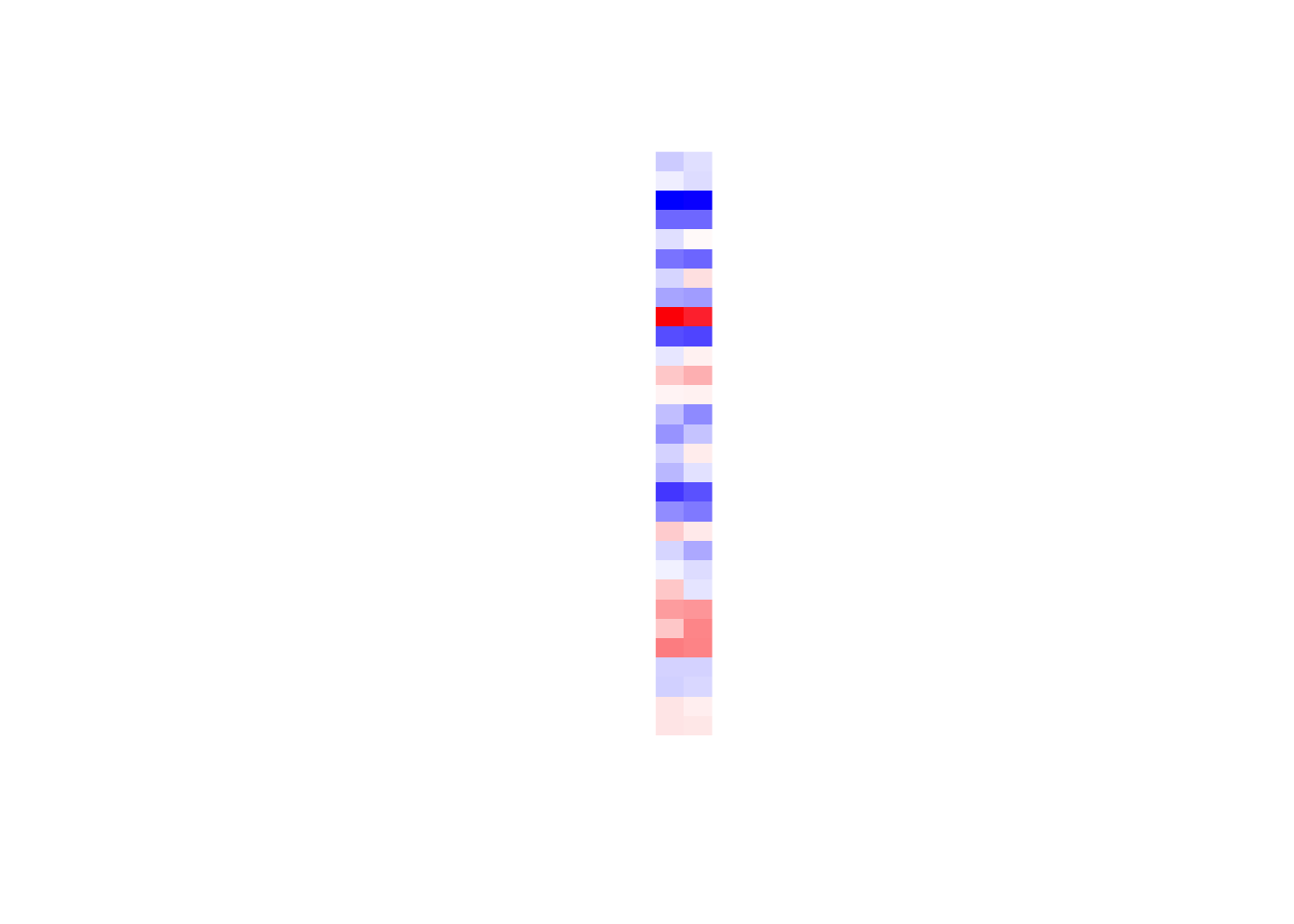
The principal components are the columns of the rotation \(U^T Y\)
PC1 = s$u[,1] * s$d[1]
PC2 = s$u[,2] * s$d[2]
plot(PC1, PC2,xlim=c(-3,3), ylim=c(-3,3))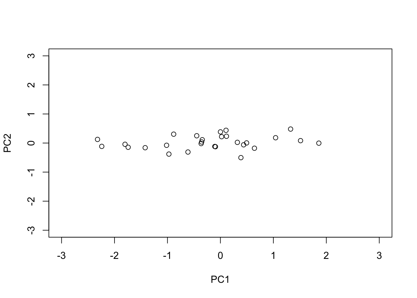
The fat matrix
n = 100
y_fat = t(y)
s = svd(y_fat)
plot.matrix(y_fat,asp=1/20)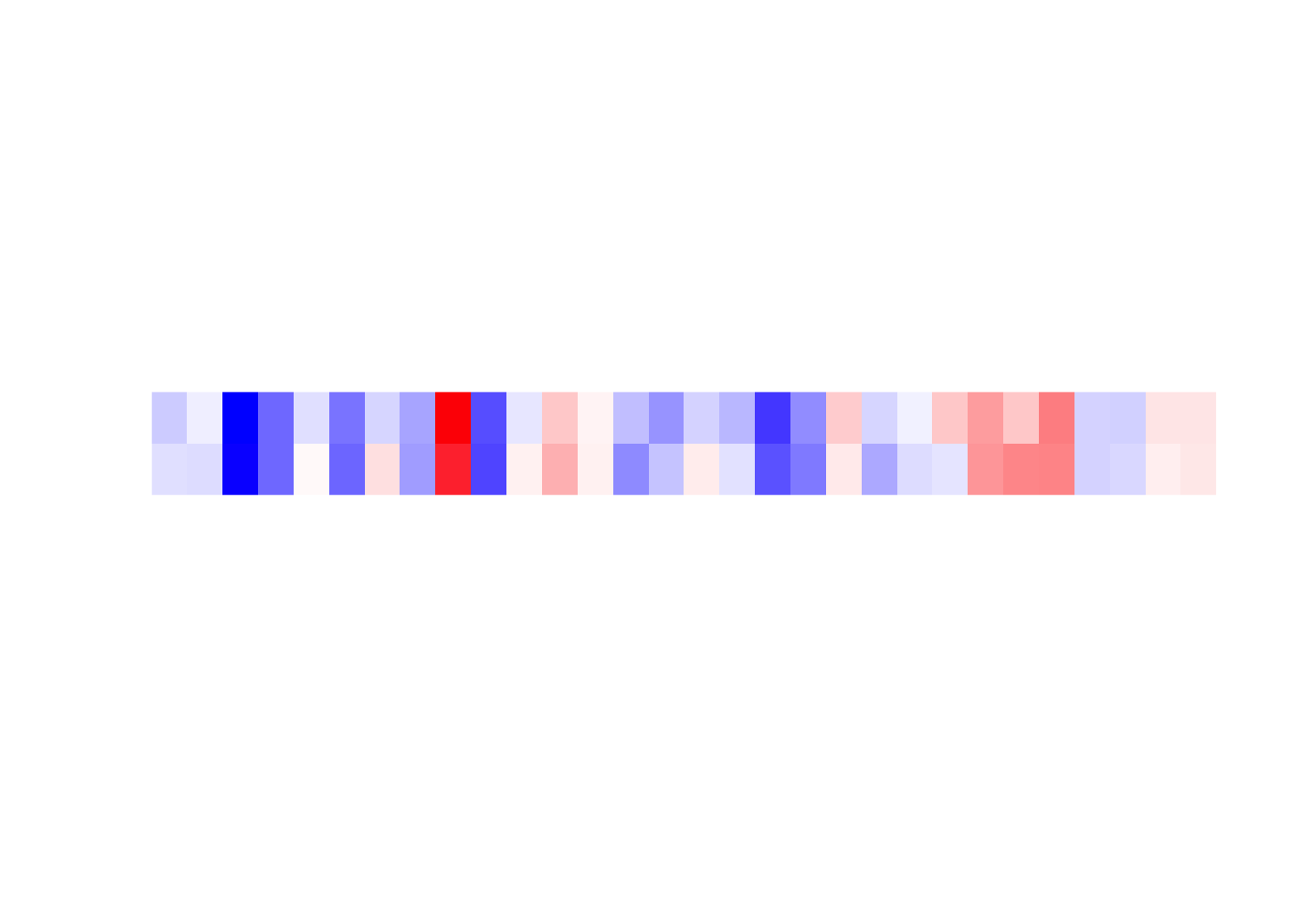
The principal components are the columns of the rotation \(U^T Y\)
PC1_fat = s$d[1] * s$v[,1]
PC2_fat = s$d[2] * s$v[,2]
plot(PC1_fat, PC2_fat,xlim=c(-3,3), ylim=c(-3,3))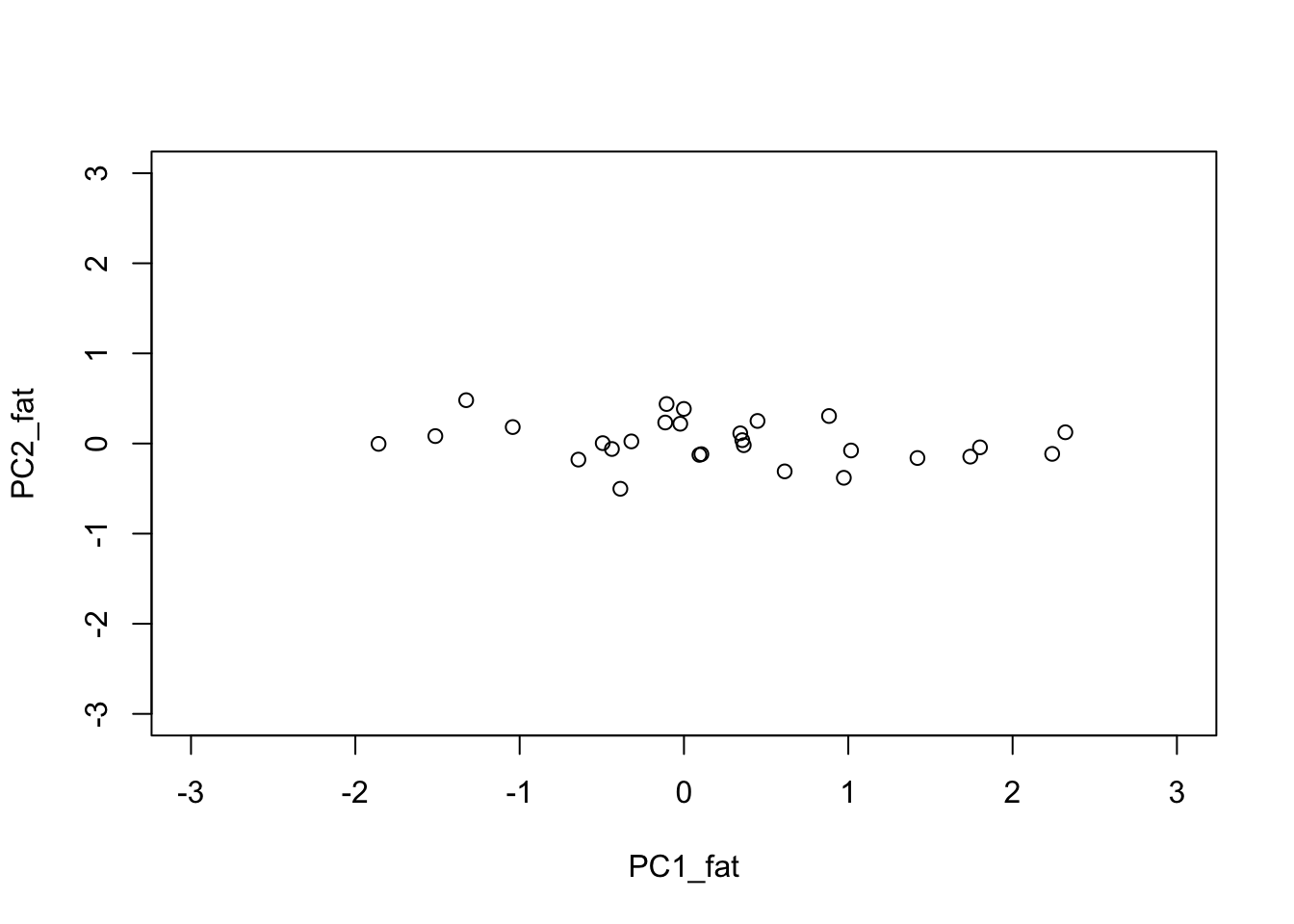
par(mfrow=c(1,2))
plot(PC1,PC2,xlim=c(-3,3),ylim=c(-3,3), main='thin Y')
plot(PC1_fat,PC2_fat,xlim=c(-3,3),ylim=c(-3,3), main='fat Y')