A simple example of EM algorithm
The gist of EM
- Initialize paramters \(\theta\)
- E-step: Calculate the likelihood \(P(Z | X, \theta)\), \(Z\) is hidden variable
- M-step: Maximize the conditional expectation of \(ln P(X,Z | \theta)\), i.e
\[ \DeclareMathOperator*{\argmax}{argmax} \theta_{n+1} \leftarrow \argmax_{\theta} \mathbf{E}_{Z|X,\theta}\{ \ln P(X,Z | \theta) \} \]
Simulate data
REAL_ALPHA = 0.7
REAL_THETAS = c(0.8, 0.45)
Give two coins A and B with the probability of getting heads \(\theta_A = 0.8\) and \(\theta_B = 0.45\)
The data below is generated by picking either coin A or B with probability \(P(Z = A) = \alpha = 0.7\), tossing it 10 times and recording 1 for head, 0 for tail. Repeat this process 5 times to obtain a total number of 50 coin tosses.
## 1211122| 1 | 1 | 1 | 1 | 1 | 1 | 1 | 1 | 0 | 1 |
| 0 | 1 | 0 | 1 | 1 | 0 | 1 | 0 | 0 | 1 |
| 1 | 1 | 1 | 0 | 1 | 1 | 1 | 1 | 0 | 1 |
| 0 | 0 | 0 | 1 | 0 | 1 | 1 | 1 | 1 | 0 |
| 1 | 1 | 1 | 1 | 0 | 1 | 0 | 1 | 1 | 1 |
| 0 | 0 | 0 | 0 | 0 | 0 | 0 | 0 | 1 | 0 |
| 0 | 1 | 0 | 1 | 1 | 0 | 0 | 1 | 0 | 1 |
Normally all we could observe is the sequences of heads and tails without knowing which coins each sequence came from.
Step-by-step
The likelihood of each coin
Let \(X\) be the number of heads and \(Z\) the identity of the coin. The probability of observing \(x\) heads after \(n\) tosses is
\[ P(X = x | Z = z) = {n \choose x}\theta_z^{x} (1 - \theta_z)^{n - x} \]
normalize.vec <- function(x) {
    return(x/sum(x))
}

p_z_given_x <- function(params, x) {
    n = length(x)
    heads = sum(x)
    p_coin = c(params[1], 1 - params[1])
    p_head = params[-1]
    # (n choose x) is canceled out
    sapply(1:length(p_head), function(i) {
        p = p_head[i]
        (p^heads) * (1-p)^(n - heads) * p_coin[i]
    }) %>%
        normalize.vec() %>%
        return()
}
E-step
For each observed sequence, calculate the likelihood that it comes from coin \(z\),
\[ Q_i = P(Z | X_i, \theta) = \begin{cases} \frac{(\theta_A)^{x} (1 - \theta_A)^{10-x} \alpha}{(\theta_A)^{x} (1 - \theta_A)^{10-x} \alpha + (\theta_B)^{x} (1- \theta_B)^{10 - x} (1 - \alpha)} \; \text{ if }Z = A \\ \frac{(\theta_B)^{x} (1- \theta_B)^{10 - x} (1 - \alpha)}{(\theta_A)^{x} (1 - \theta_A)^{10-x} \alpha + (\theta_B)^{x} (1- \theta_B)^{10 - x} (1 - \alpha)} \; \text{ if }Z = B \end{cases} \]
thetas_guess = runif(3)
print(thetas_guess)
## [1] 0.06102840 0.55951562 0.05163475# P(X | thetas)
pZ.X = sapply(1:nrow(data), function(i) {
obs = data[i,]
# print(obs)
return(p_z_given_x(thetas_guess, obs))
}) %>%
t() %>%
set_colnames(c('P(Z = A | x_i)', 'P(Z = B | x_i)'))
pZ.X## P(Z = A | x_i) P(Z = B | x_i)
## [1,] 0.9999999839 1.608178e-08
## [2,] 0.9952583322 4.741668e-03
## [3,] 0.9999996248 3.751883e-07
## [4,] 0.9952583322 4.741668e-03
## [5,] 0.9999996248 3.751883e-07
## [6,] 0.0007080044 9.992920e-01
## [7,] 0.9952583322 4.741668e-03M-step
\[ \DeclareMathOperator*{\sum}{\Sigma} \begin{align} \alpha^{t + 1} &\leftarrow& \frac{\sum_i Q_i(Z = A)}{N} \\ \theta^{t+1}_A &\leftarrow& \frac{\sum_i Q_i(Z = A)x_i}{N\sum_i Q_i(Z = A)} \\ \theta^{t+1}_B &\leftarrow& \frac{\sum_i (1 - Q_i(Z = A)) x_i}{N \sum_i (1 - Q_i(Z=A))} \\ N = 5,\text{ i.e. number of examples} \end{align} \]
Putting together
estimate_params <- function(alpha, a, b, data, max_iter = 10, keep_track = FALSE) {
iter = 1
tracks = list()
if (keep_track) tracks = append(tracks, list(c(alpha, a, b)))
while (iter < max_iter) {
# E-step
pZ.X = sapply(1:nrow(data), function(i) {
obs = data[i,]
return(p_z_given_x(c(alpha, a, b), obs))
}) %>%
t()
# M-step
x = apply(data, 1, sum)
alpha = sum(pZ.X[,1]) / nrow(data)
a = sum(pZ.X[,1] * x) / (ncol(data) * sum(pZ.X[,1]))
b = sum(pZ.X[,2] * x) / (ncol(data) * sum(pZ.X[,2]))
if (keep_track) tracks = append(tracks, list(c(alpha, a, b)))
iter = iter +1
}
if (keep_track) return(do.call(rbind, tracks))
else return(c(alpha, a, b))
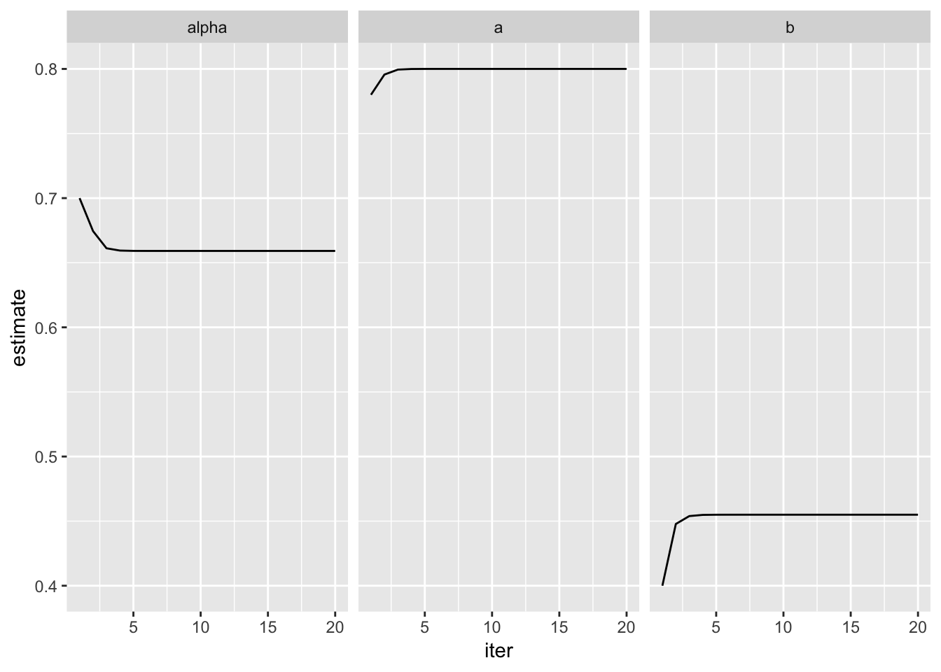
}Start with close estimates
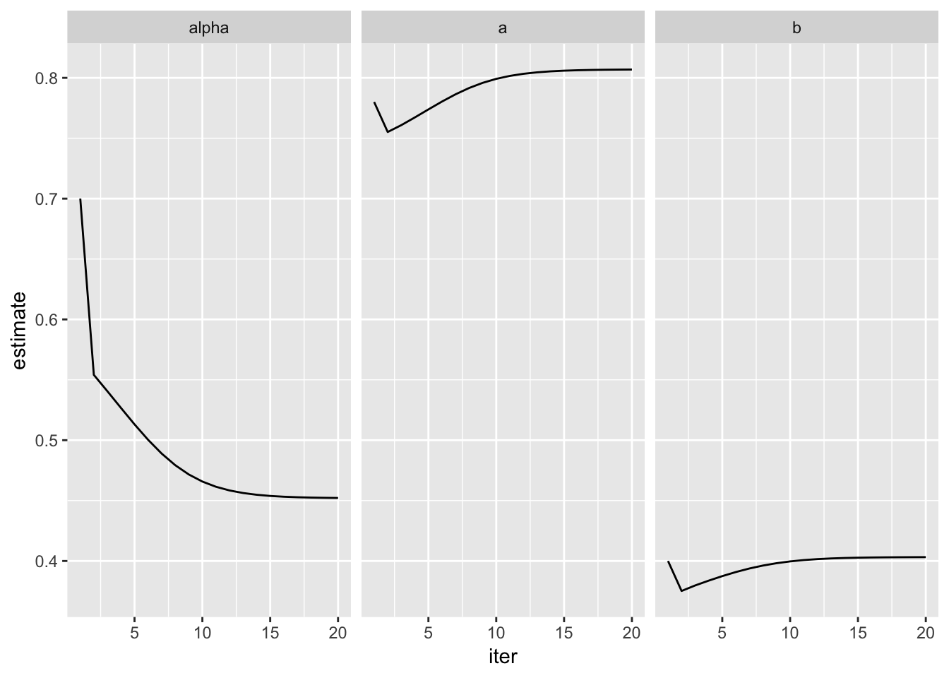
Convergence of estimated parameters from various initial positions
If the initial estimates are different enough, we may be able to see various local maxima that the algorithm converged to.
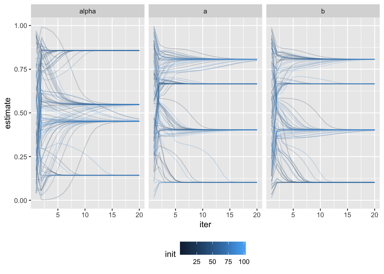
More observations
With more observations, it is reasonably expected that the estimates will be much closer to the true model.
N_SEQS = 50
N_TOSS = 50
data_big = sample(c(1, 2), size = N_SEQS, prob = c(REAL_ALPHA, 1-REAL_ALPHA), replace = TRUE) %>%
    lapply(function(coin) {
        sample(c(1,0),size = N_TOSS,replace = TRUE, prob = c(REAL_THETAS[coin], 1 - REAL_THETAS[coin]))
    }) %>%
    do.call(rbind, .)


N_ITERS = 20
N_INITS = 100
estimates_big =
    lapply(1:N_INITS, function(i) {
        inits = runif(3)
        estimate_params(inits[1], inits[2], inits[3], data = data_big, max_iter = N_ITERS, keep_track = TRUE) %>%
            cbind(rep(i, N_ITERS)) %>%
            cbind(1:N_ITERS) %>%
            set_colnames(c('alpha', 'a', 'b', 'init', 'iter')) %>%
            return()
    }) %>%
    do.call(rbind, .)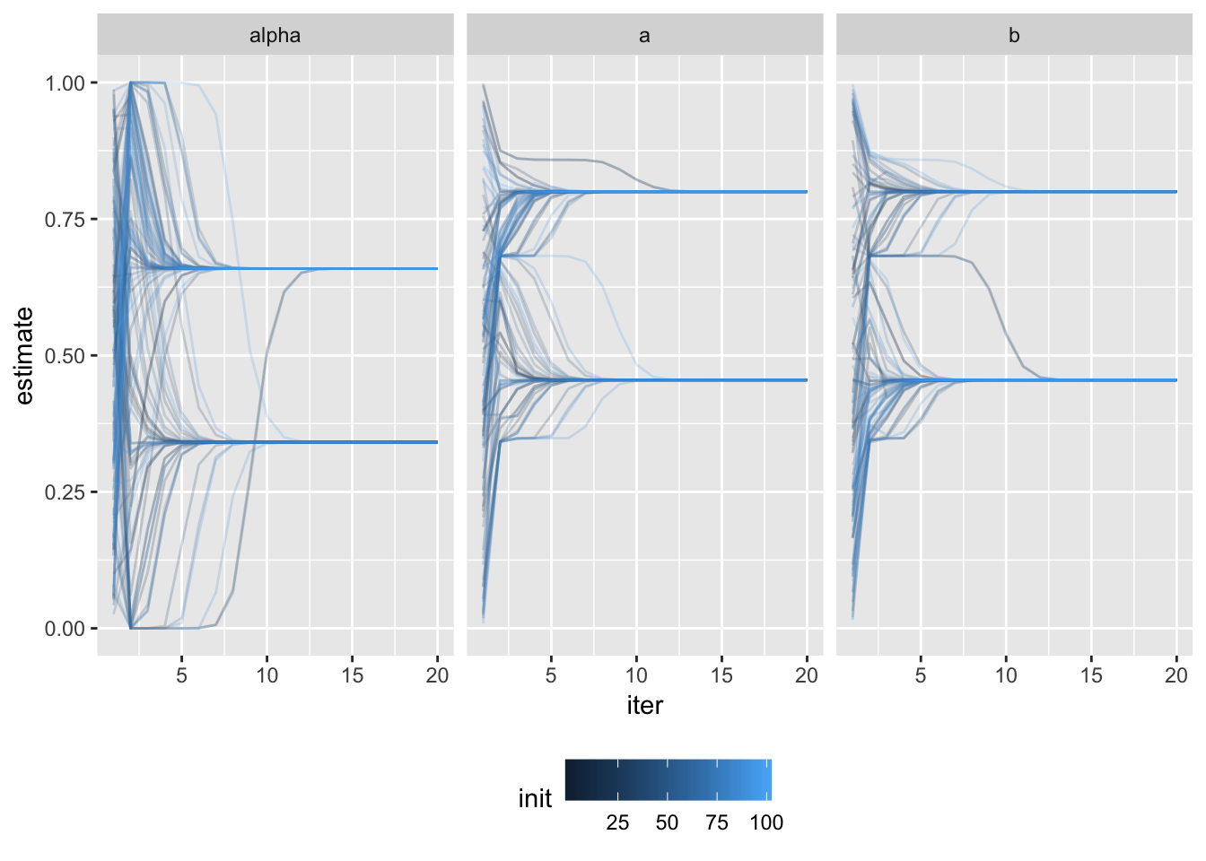
Even with very large number of observations, we can see that the algorithm has trouble converging to a single solution.
The two solutions seem to be equally good for the given data
dat.incomplete = apply(dat, 1, FUN = function(x) { return(any(is.na(x)))})
alternatives = dat[!dat.incomplete,] %>%
    kmeans(centers = 2) %>%
    `$`('centers')
alternatives
## alpha a b
## 1 0.6591312 0.8000129 0.4549742
## 2 0.3408688 0.4549742 0.8000129Start with close estimates