Importance sampling
\[ \DeclareMathOperator*{\argmax}{arg\,max} \DeclareMathOperator*{\E}{\mathbb{E}} \]
An example
The example below is taken from [1]
Let \(X\) be a random variable with uniform distribution in \([0,10]\), \[ X \sim Uniform(0,10) \]
Consider the function \(h(x) = 10 e^{-2|x-5|}\). Suppose we want to calculate \(\E_X[h(X)]\). By definition,
\[\begin{align} \E_X[h(X)] &= \int_{0}^{10} h(x) f(x)dx \\ &= \int_{0}^{10} exp(-2|x-5|) dx \end{align}\]A straightforward way to do this is sampling \(X_i\) from the uniform(0,10) density and calculating the mean of \(10\cdot h(X_i)\)
X <- runif(100000,0,10)
Y <- 10*exp(-2*abs(X-5))
c(mean(Y), var(Y))
## [1] 0.9968198 3.9740918If we look at \(h(X)\) more closely, it turns out \(h(X)\) is peaked at 5. It means when we sample \(X_i\) from \(Uniform(0,10)\), most of the time \(X_i\) will fall out of the peak area and contribute nothing to the integral.
h <- function(x) {
    return( 10*exp(-2*abs(x-5)) )
}
x <- (0:200)/20
plot(x, h(x), type='l',col='blue')
lines(x,dunif(x, 0, 10), col='red')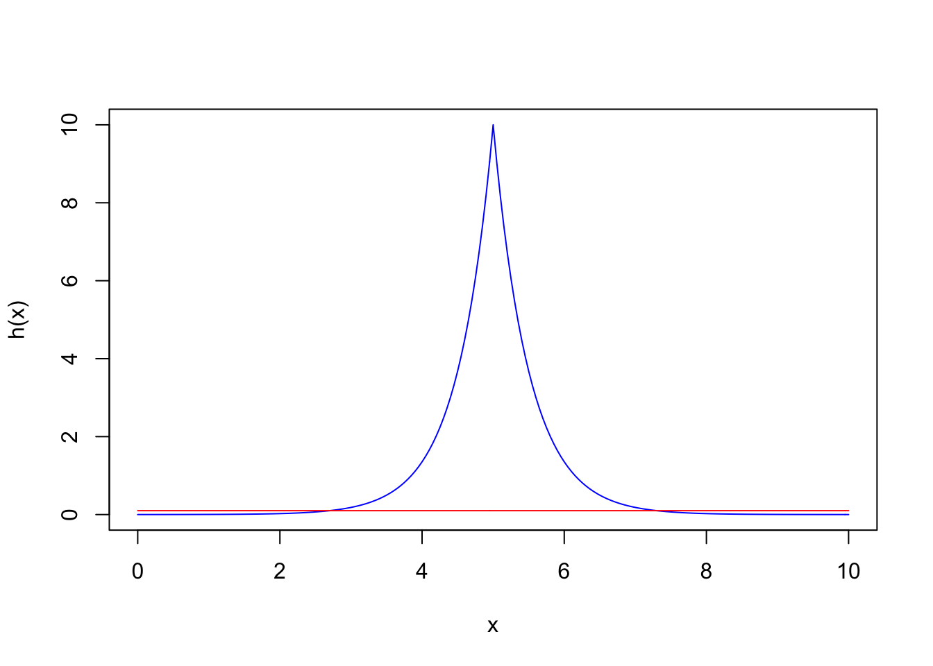
Is there a more efficient way to sample \(X_i\)? Looks like we can sample \(X_i\) efficiently from a normal distribution centered at 5. And yes, we’ll have to adjust the integrand so that it removes the sampling bias.
X <- rnorm(100000, mean=5, sd=1)
Y <- h(X)* dunif(X, 0, 10) / dnorm(X, mean=5, sd=1)
c(mean(Y), var(Y))
## [1] 0.9999021 0.3575852The estimate \(\E_X[h(X)]\) is the same, with much smaller variance, because we were able to sample more \(X_i\) in the important region.
Formalization
The example above exemplifies one among many uses of importance sampling which is a method to generate rare, or not-so-often, events to improve the precision, or to make possible some empirical calculations on random variable.
\[\begin{align} \E_X[h(X)] &= \int_D h(x) f(x) dx \quad,\quad f(x)\text{is the density function} \\ &= \int \frac{h(x) f(x)}{g(x)} g(x) dx \end{align}\]Now if \(g(x)\) is a density function and \(g(x) > 0 \;\forall x \in D\), the integrand can be re-arranged
\[\begin{align} \E_X[h(X)] &= \int \frac{h(x) f(x)}{g(x)} g(x) dx \\ &= \E_Y\left[ \frac{h(Y) f(Y)}{g(Y)}\right] \end{align}\]It seems the random variable \(X\) has magically morphed into \(Y\). It is just a way to distinguish the two distributions characterized by different density functions \(f\) and \(g\). It implies that we can now sample from the distribution of \(Y\) instead of the original \(X\), and the adjustment term \(\frac{f(x)}{g(x)}\) is call importance function.
References
[1] J. Goldstick, “Importance Sampling,” Statistics 406. http://dept.stat.lsa.umich.edu/~jasoneg/Stat406/lab7.pdf, 2009.

