Parallel Pearson Correlation
Motivation
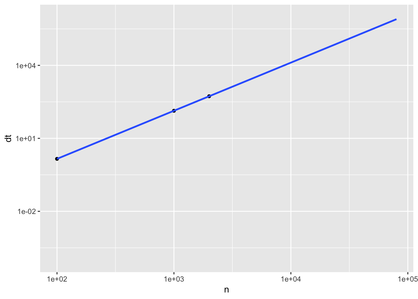
Let’s look at the time it takes to calculate all pairwise correlation for \(n\) variable, with \(m\)=200 samples.
| n | dt |
|---|---|
| 1e+02 | 1.433043e+00 |
| 1e+03 | 1.359290e+02 |
| 2e+03 | 5.371534e+02 |
| 1e+05 | 1.230446e+06 |
Given the timing above, and the extrapolated timing for \(10^{5}\) genes, which is roughly the order of number of genes/transcripts in a transcriptomic profile, it would take 14.2412778 days to finish the calculation. We can save some more time, by only calculating half of the pairs (since \(cor(A,B) = cor(B,A)\)). The computing time is still beyond the patience of an average scientist. Let’s see how much parallelization can help.
Parallelization
mat = MASS::mvrnorm(n=200,mu = rep(1,3),
                    Sigma = matrix(c(1, 0.2, 0.7,
                                     0.2, 1, 0.2,
                                     0.7, 0.2, 1), nrow=3))
Simple parallelization: one variable per worker
In this approach we’ll distribute one column (variable) to each worker available, thus we can scale to at max \(n\) workers, each will calculate \(n\) correlation coefficient.
# nCores = detectCores() -2
parCor.1 = function(mat,Ncpus=2) {
    output =
    (parSapply(cl= makeCluster(Ncpus),
              X=1:ncol(mat),
              FUN = function(i) {
        return(sapply(1:ncol(mat), FUN = function(j) {
            return(cor(mat[,i],mat[,j]))
        }))
    })
    )
    return(output)
}
# parCor.1(mat,nCores)
Speed-up
timing.ser[,'nCpus'] = 1
timing = rbind(timing.ser, timing.par)
ggplot(timing, aes(x=n,y=dt,group=nCpus)) +
    scale_x_log10() +
    scale_y_log10() +
    geom_line(aes(color=factor(nCpus))) +
    geom_point(aes(color=factor(nCpus)))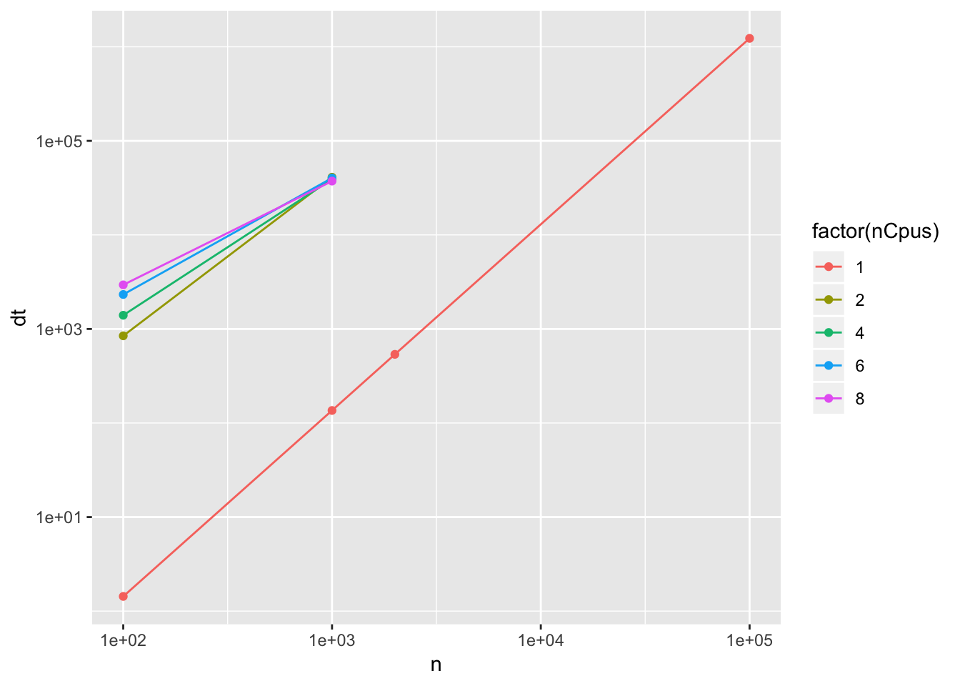
Unfortunately this parallization scheme is not working. The speed-up gained at doubling the cores is actually less than 1: the parallel version is much slower than the serial computation.
timing[,'speedUp'] = 1
for (i in 1:nrow(timing)) {
    n = timing[i,'n']
    reftime = timing[timing[['n']] == n & timing[['nCpus']] == 1, 'dt']
    timing[i,'speedUp'] = reftime / timing[i,'dt']
}
knitr::kable(timing)| n | dt | nCpus | speedUp |
|---|---|---|---|
| 1e+02 | 1.433043e+00 | 1 | 1.0000000 |
| 1e+03 | 1.359290e+02 | 1 | 1.0000000 |
| 2e+03 | 5.371534e+02 | 1 | 1.0000000 |
| 1e+05 | 1.230446e+06 | 1 | 1.0000000 |
| 1e+02 | 8.453151e+02 | 2 | 0.0016953 |
| 1e+03 | 4.105283e+04 | 2 | 0.0033111 |
| 1e+02 | 1.398747e+03 | 4 | 0.0010245 |
| 1e+03 | 3.915751e+04 | 4 | 0.0034713 |
| 1e+02 | 2.325909e+03 | 6 | 0.0006161 |
| 1e+03 | 4.027128e+04 | 6 | 0.0033753 |
| 1e+02 | 2.944231e+03 | 8 | 0.0004867 |
| 1e+03 | 3.734735e+04 | 8 | 0.0036396 |
The curse of I/O
Assuming we eventually have a large enough matrix so that the parallization overhead become smaller compared to that of the performance gain, there is yet another problem when the matrix is too large. Each thread will try to create a copy of the big input matrix, thus quickly draining the system memory. The resulted correlation matrix is a large one, too. For example, it takes 37.252903 gigabytes to store a \(10^5 \times 10^5\) matrix in which each element is a 32-bit float. We can go a bit further to retain only the upper (or lower) triangular matrix to reduce the matrix size by half. Even so, the memory requirement is still somewhat beyond an average machine like a laptop (unless you’re on a really decent one). It means you’ll need to write the output to disk at some point.
A simple approach is to write every column to disk, and read them back up into a matrix when you need them. For the sake of being organized, we can go one step further by consolidating the result into an upper triangular matrix, and write the result in that form. The regular way of handling these I/O might not be sufficient for this task.
Massive parallel: chunk of pairs per worker
In this approach we’ll treat every pair as a compute job, key them with a unique index, send to any compute unit available, and put them back into the result matrix using their key. This approach can be implemented easily with spark, but the necessary functions are not yet ported to sparkR, at the time of this writing.

