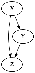
Directed Acyclic Graph and conditional independence

Analytical estimation of probabilities

The conditional probability \[ \begin{align} P(Z = 1 \vert Y = 1) &= \frac{1}{2} \left[ \frac{e^2}{1 + e^2} + \frac{e}{1 + e} \right] \\ &= 0.4156266 \end{align} \]

Empirical solution

pYgivenX <- function(y,x) {
    p1 = exp(4*x - 2) / (1 + exp(4*x-2))
    if (y==1) return(p1)
    else return(1-p1)
}

pZgivenXY <- function(z,x,y) {
    p1 = exp(2*(x+y) -2) / (1 + exp(2*(x+y) -2))
    if (z ==1) return(p1)
    else return(1-p1)
}

rbanana <- function(n) {
    output = matrix(rep(0,n*3),nrow=n)
    # generate X, Y and Z
    output[,1] <- rbinom(n,size=1,prob=0.5)
    output[,2] <- rbinom(n,size=1,pYgivenX(1,output[,1]))
    output[,3] <- rbinom(n,size=1,pZgivenXY(1,output[,1],output[,2]))
    return(output)
}

N = 1:50 * 100
V = sapply(N, FUN = function(x) {
    v =  rbanana(x)
    return(sum(v[v[,2] == 1,3]) *1. / x )
})

lm.pzy = lm(V[25:50] ~ N[25:50])

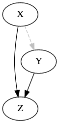
Intervention

Suppose we fix \(Y\) at the value \(y=1\). Such intervention results in the new joint probability

\[\begin{align} f^*(x,z) &= f(x) f(z \vert x) \end{align}\]

and thus the marginal distribution

\[\begin{align} f^*(z) &= \sum_{x} f(x) f(z\vert x) \end{align}\]

i.e.

\[\begin{align} Z \sim Bernoulli \left( \frac{e^{2x}}{1 + e^{2x}} \right) \end{align}\]

\[\begin{align} P(Z = 1 | Y:= 1) &= \frac{1}{2}\left(\frac{e^0}{1 + e^0}\right) + \frac{1}{2}\left( \frac{e^{-2}}{1 + e^{-2}}\right) \\ &= \end{align}\] 0.6903985

The simulation result is generated by the function call

rbanana.givenY <- function(n,y) {
    output = matrix(rep(0,n*3),nrow=n)
    # Fix Y
    output[,2] <- y
    output[,1] <- rbinom(n,size=1,prob=0.5)
    output[,3] <- rbinom(n,size=1,pZgivenXY(1,output[,1],output[,2]))
    return(output)
}

Under this intervention of \(Y=1\), the empirical estimation of \(P(Z = 1 \vert Y := 1)\) = 0.6707593

Conditioning by observation

\[ \begin{align} \newcommand{\intf}{\int_{-\infty}^{+\infty}} f(z \vert y) &= \intf f(z \vert y,x) f(x \vert y) dx \\ &= \intf f(z \vert y,x) f(x) dx \quad \text{(since X is not dependent on Y)} \\ &= \intf \frac{1}{\sqrt{2\pi}} \exp\left(-\frac{(z - \beta y - \gamma x)^2}{2}\right) \frac{1}{\sqrt{2\pi}}\exp\left( - \frac{x^2}{2}\right) dx \\ &= \frac{1}{2\pi} \intf \exp\left( - \frac{x^2 + \gamma^2 x^2 - 2\gamma(z - \beta y)x + (z - \beta y)^2}{2} \right) dx \end{align} \] Gaussian integral [1] gives

\[ \begin{align} \int_{-\infty}^{\infty} e^{-ax^2 + bx + c} dx = \sqrt{\frac{\pi}{a}} e^{ \frac{b^2}{4a} + c} \tag{1} \end{align} \]

In the expression of \(f(z\vert y)\), \[ \begin{align} a &= \frac{1 + \gamma^2}{2} \\ b &= \gamma(z - \beta y) \\ c &= -\frac{(z - \beta y)^2}{2} \end{align} \] thus, \[ \begin{align} f(z\vert y) = \frac{1}{\sqrt{2\pi(1 + \gamma^2)}} \exp\left( -\frac{(z-\beta y)^2}{2 (1 + \gamma^2)} \right) \end{align} \] or equivalently, \[ \begin{align} Z\vert Y=y \sim Normal(\beta y, 1 + \gamma^2) \end{align} \] \[ \begin{align} \E{Z \vert Y = y} &= \int z f(z \vert y) dz \\ &= \beta y \end{align} \]

Conditioning by intervention

When there is intervention on \(Y\), i.e, \(Y := y\), the joint distribution becomes that of \((X,Z)\).

\[ \begin{align} f^*(x,z) &= f(z | x,y) f(x) \\ f(z | Y := y) = f^*(z) &= \intf f(z | x,y) f(x) dx \end{align} \]

which happens to be the same as \(f(z \vert Y = y)\) derived above. However, since \(Y\) is chosen in experimental settings, \(f(y)\) is determined by the experimental process. If we assume that in the experiment, \(Y \sim Normal(\mu_Y,1)\)

\[ \begin{align} \E{Z \vert Y:=y } = \intf z f(z\vert Y:= y) dy \end{align} \]

Joint distribution of \((Y,Z)\)

\[ \begin{align} f(y,z) &= \intf f(z\vert y,x) f(y \vert x) f(x) dx \\ &= \frac{1}{(\sqrt{2\pi})^3} \intf \exp\left( - \frac{x^2 + (y- \alpha x)^2 + (z - \beta y - \gamma x)^2}{2}\right) dx \\ &= \frac{1}{(\sqrt{2\pi})^3} \intf \exp\left( -\color{red}{\frac{(1 + \alpha^2 + \gamma^2)}{2}}x^2 + \color{blue}{(\alpha y - \beta y + z)}x + \color{green}{\frac{- y^2 - (z - \beta y)^2}{2}}\right) dx \\ &= \frac{1}{(\sqrt{2\pi})^3} \sqrt{ \frac{2\pi}{1 + \alpha^2 +\gamma^2}} \exp \left(\frac{((\alpha - \beta)y + z)^2}{2(1 + \alpha^2 + \gamma^2)}- \frac{y^2 + (z-\beta y)^2}{2}\right) \\ &= \frac{1}{2\pi\sqrt{1 + \alpha^2 + \gamma^2}}\exp\left(\dots\right) \tag{2} \end{align} \]

Based on the form of \(f(y,z)\) in (2), we may guess that \((Z,Y) \sim Normal(\vector{\mu},\matrix{\Sigma})\) follow some bivariate normal distribution which has the form [2]

\[ \begin{align} f(x,y) = \frac{1}{2\pi\sigma_X\sigma_Y\sqrt{1 - \rho^2}} \exp\left( - \frac{1}{2 (1-\rho^2)}\left[ \frac{(x - \mu_X)^2}{\sigma^2_X} + \frac{(y - \mu_Y)^2}{\sigma^2_Y} - \frac{2\rho(x-\mu_X)(y - \mu_Y)}{\sigma_X\sigma_Y}\right]\right) \tag{3} \end{align} \]

We’ll skip the derivation of (3) from (2), and use simulation to explore this distribution.

Simulation of joint distribution \((Z,Y)\)

Assuming the following parameter values

• \(\alpha =\) 0.2
• \(\beta =\) -0.2
• \(\gamma =\) 0.2

rstrawberry <- function(n,alpha, beta, gamma) {
    output = matrix(rep(0,n*3),nrow=n)
    # generate X, Y and Z
    output[,1] <- rnorm(n,mean = 0,sd = 1)
    output[,2] <- rnorm(n,mean=output[,1] *alpha, sd = 1 )
    output[,3] <- rnorm(n,mean=output[,2] *beta + output[,3]*gamma, sd=1)
    return(output)   
}

rstrawberry.givenY <- function(n,y, alpha, beta, gamma) {
    output = matrix(rep(0,n*3),nrow=n)
    # generate X, Y and Z
    output[,1] <- rnorm(n,mean = 0,sd = 1)
    output[,2] <- y
    output[,3] <- rnorm(n,mean=output[,2] *beta + output[,3]*gamma, sd=1)
    return(output)   
}

## Warning: Computation failed in `stat_density2d()`:
## bandwidths must be strictly positive

## Warning in cor(x = V.cont[, "Y"], y = V.cont[, "Z"]): the standard
## deviation is zero

knitr::kable(data.frame(list("Setting"=c("Observation", "Intervention"),
                             "Correlation"= c(corr.yz.obs, corr.yz.int))))