Fitting negative binomial distribution and goodness-of-fit
The package MASS provides a function, fitdistr to fit an observation over discrete distribution using Maximum likelihood.
Obtaining data
We first need to generate some data to fit. The rnegbin(n,mu,theta) function can be used to generate n samples of negative binomial with mean mu and variance mu + mu^2 / theta. To describe the distribution in terms of \(r\) (number of successes) and \(p\) (probability of success), we need to derive these parameters from the properties of \(NB\) distribution, i.e.
\[ \begin{align} r &= \frac{\mu p}{1 - p} = \theta \\ p &= \frac{\theta}{\mu + \theta} \end{align} \]
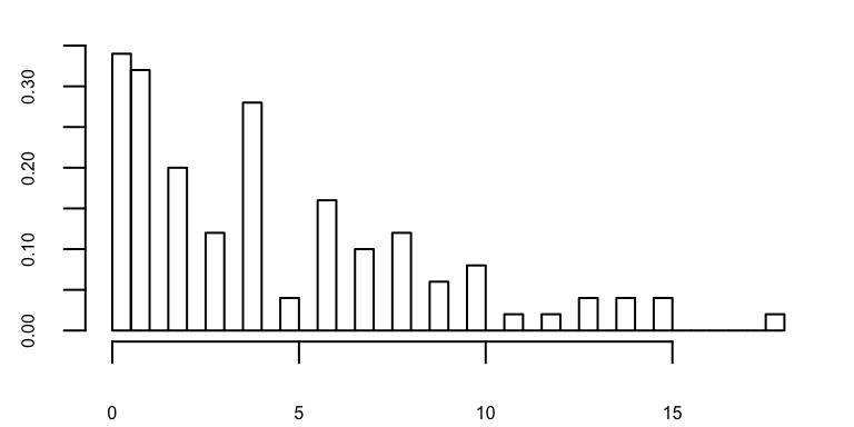
In the example below, we sample \(X\) from a negative binomial distribution with * mean \(\mu=\) 5 * variance \(\sigma^2 = \mu + \mu^2/\theta,\, \theta=\) 1
or equivalently
\(X \sim NB(r=\) 1\(,p=\) 0.1666667\()\)
Fitting with pre-determined distribution
If we know \(X \sim NB(r,p)\), we can fit the data using this distribution.
x_plot = seq(0, 100,1)
nbfit = fitdistr(x,'negative binomial')
nbfit
## size mu
## 1.1955179 4.4299973
## (0.2341407) (0.4565670)The fitted model contains 2 parameters, which can be converted to our conventional \((r,p)\) as following
r.fit = nbfit$estimate['size']
p.fit = r.fit / (nbfit$estimate['mu'] + r.fit)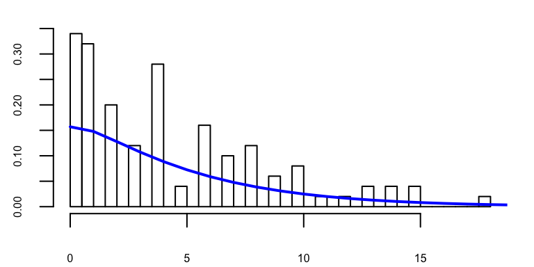
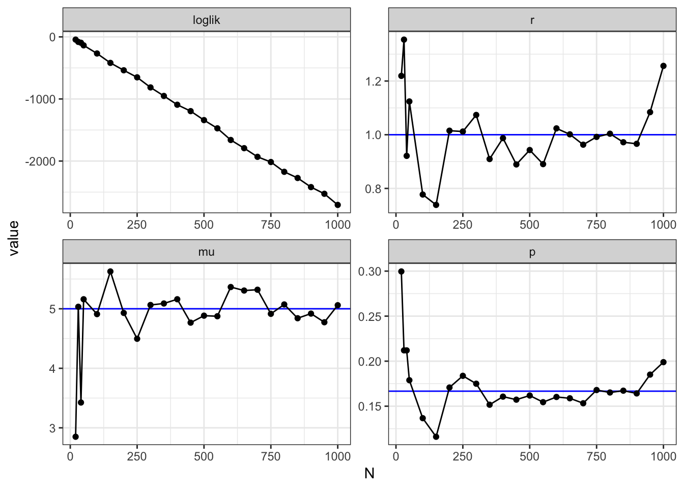
The effects of sample size
Conventional wisdom tells us that the more samples we have, the better we should be able to infer, i.e. the less error we make. When the number samples increase, we should expect the inferred parameters to approach the true value. The graphs below clearly illustrate that when the number of samples increases * Log-likelihood approaches zero, i.e. the more confident we are * \((r,p)\) approach the true values
Goodness-of-fit
What if we don’t know the distribution of \(X\) before hand? There are multiple statistical hypothesis tests to evaluate whether a distribution is good for fitting a data set, for example Shapiro-Wilk for normality, Anderson-Darling for a given distribution…
Assuming Poisson distribution
We’ll explore how the Pearson chi-squared test can tell if a distribution, e.g. Poisson can properly describe our data set.
\[ \chi^2 = \sum_{i=1}^{n}\frac{(O_i - E_i)^2}{E_i} \] where * \(O_i\) is the observed frequency in bin \(i\) * \(E_i\) is the expected frequency for bin \(i\)
We want to test whether
\[ \begin{align} H_0 \equiv X \sim Poisson(\lambda) \\ \lambda = \mu \end{align} \]
Under \(H_0\), the outcome of \(X\) would be
nsamples = length(x)
f.obs = table(x)
bins = as.numeric(names(f.obs))
f.hyp = dpois(bins,lambda = mu)*nsamples
chiSquare.pois = sum((f.obs-f.hyp)^2/f.hyp)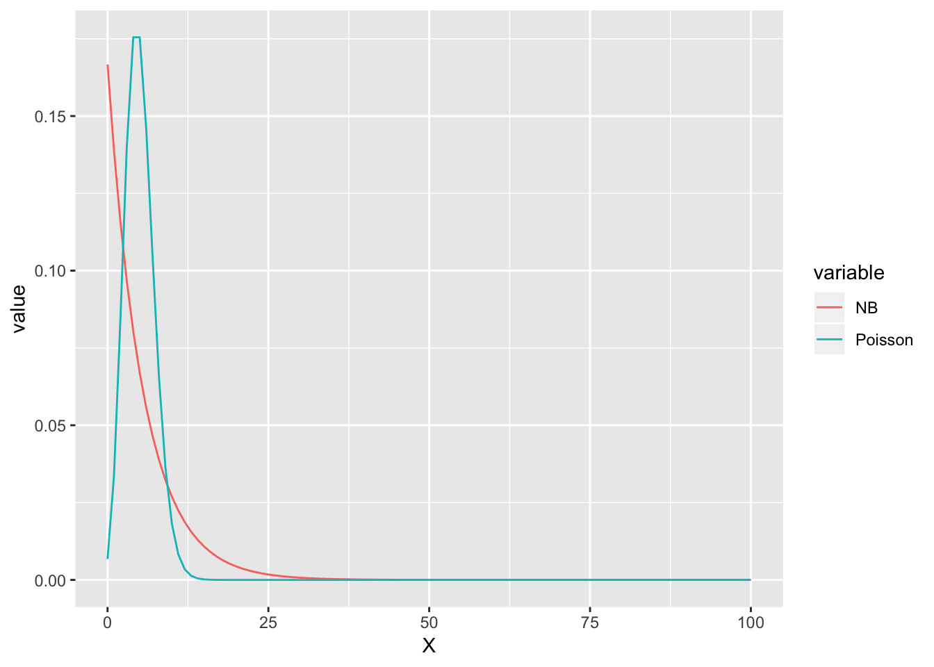
Assuming NB distribution
nsamples = length(x)
f.obs = table(x)
bins = as.numeric(names(f.obs))
f.hyp = dnbinom(bins,size=r.fit,prob=p.fit)*nsamples
chiSquare.nb = sum((f.obs-f.hyp)^2/f.hyp)
dof = length(bins) - 1
The goodness-of-fit for each distribution is determined by consulting the \(\chi^2\) distribution with 32 degree-of-freedom.
| Distribution | chi-squared | P(chi.sq) |
|---|---|---|
| Poisson | 5.400142e+14 | 0.000000e+00 |
| Negative binomial | 9.787575e+01 | 4.717345e-09 |
In other words, it’s extremely unlikely that \(X \sim Poisson(\lambda=\) 5 \()\) (Prob = 0 ). The decision with \(H_0 \equiv X \sim NB(r =\) 1 \(, p=\) 0.1666667 \()\) is a bit more difficult, depending on our choice of threshold. In fact it seems this goodness-of-fit test does not do a good job in telling good fit from a bad one.

